by M. Bourne

Interactive exploration

See an applet where you can explore Simpson’s Rule and other numerical techniques:
Riemann Sums Applet

In the last section, Trapezoidal Rule, we used straight lines to model a curve and learned that it was an improvement over using rectangles for finding areas under curves because we had much less “missing” from each segment.

We seek an even better approximation for the area under a curve.

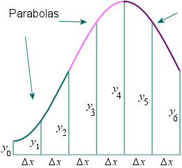
In Simpson’s Rule, we will use parabolas to approximate each part of the curve. This proves to be very efficient since it’s generally more accurate than the other numerical methods we’ve seen. (See more about Parabolas.)

We divide the area into $displaystyle{n}$n equal segments of width $displaystyleDelta{x}$Δx. The approximate area is given by the following.

Simpson’s Rule

Area $displaystyle={int_{{a}}^{{b}}} f{{left({x}right)}}{left.{d}{x}right.}$=∫ab​f(x)dx

$displaystyleapproxfrac{{Delta{x}}}{{3}}{left({y}_{{0}}+{4}{y}_{{1}}+{2}{y}_{{2}}+{4}{y}_{{3}}+{2}{y}_{{4}}+right.}$≈3Δx​(y0​+4y1​+2y2​+4y3​+2y4​+ $displaystyle{left.ldots+{4}{y}_{{{n}-{1}}}+{y}_{{n}}right)}$…+4yn−1​+yn​)

where $displaystyleDelta{x}=frac{{{b}-{a}}}{{n}}$Δx=nb−a​

Note: In Simpson’s Rule, n must be EVEN.

See below how we obtain Simpson’s Rule by finding the area under each parabola and adding the areas.

We can re-write Simpson’s Rule by grouping it as follows:

$displaystyle{int_{{a}}^{{b}}} f{{left({x}right)}}{left.{d}{x}right.}$∫ab​f(x)dx $displaystyleapproxfrac{{Delta{x}}}{{3}}{left[{y}_{{0}}+{4}{left({y}_{{1}}+{y}_{{3}}+{y}_{{5}}+ldotsright)}right.}$≈3Δx​[y0​+4(y1​+y3​+y5​+…) $displaystyle{left.+{2}{left({y}_{{2}}+{y}_{{4}}+{y}_{{6}}+ldotsright)}+{y}_{{n}}right]}$+2(y2​+y4​+y6​+…)+yn​]

This gives us an easy way to remember Simpson’s Rule:

$displaystyle{int_{{a}}^{{b}}} f{{left({x}right)}}{left.{d}{x}right.}$∫ab​f(x)dx $displaystyleapproxfrac{{Delta{x}}}{{3}}{left[text{FIRST}+{4}{left(text{sum of ODDs}right)}right.}$≈3Δx​[FIRST+4(sum of ODDs) $displaystyle{left.+{2}{left(text{sum of EVENs}right)}+text{LAST}right]}$+2(sum of EVENs)+LAST

Approximate $displaystyle{int_{{2}}^{{3}}}frac{{{left.{d}{x}right.}}}{{{x}+{1}}}$∫23​x+1dx​ using Simpson’s Rule with $displaystyle{n}={4}$n=4.

We haven’t seen how to integrate this using algebraic processes yet, but we can use Simpson’s Rule to get a good approximation for the value.

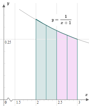
Here is the situation.

$displaystyle{y}_{{1}}= f{{left({a}+Delta{x}right)}}= f{{left({2.25}right)}}$y1​=f(a+Δx)=f(2.25) $displaystyle=frac{1}{{{2.25}+{1}}}={0.3076923}$=2.25+11​=0.3076923

$displaystyle{y}_{{2}}= f{{left({a}+{2}Delta{x}right)}}= f{{left({2.5}right)}}$y2​=f(a+2Δx)=f(2.5) $displaystyle=frac{1}{{{2.5}+{1}}}={0.2857142}$=2.5+11​=0.2857142

$displaystyle{y}_{{3}}= f{{left({a}+{3}Delta{x}right)}}= f{{left({2.75}right)}}$y3​=f(a+3Δx)=f(2.75) $displaystyle=frac{1}{{{2.75}+{1}}}={0.2666667}$=2.75+11​=0.2666667

$displaystyle{y}_{{4}}= f{{left({b}right)}}= f{{left({3}right)}}$y4​=f(b)=f(3) $displaystyle=frac{1}{{{3}+{1}}}={0.25}$=3+11​=0.25

So

Area $displaystyle={int_{{a}}^{{b}}} f{{left({x}right)}}text{d}{x}$=∫ab​f(x)dx

1. The actual answer to this problem is 0.287682 (to 6 decimal places) so our Simpson’s Rule approximation has an error of only 0.00036%.

2. In this example, the curve is very nearly parabolic, so the 2 parabolas shown above practically merge with the curve $displaystyle{y}=frac{1}{{{x}+{1}}}$y=x+11​.